XYZ Example

In this tutorial we load an XYZ trajectory.

[1]:

%matplotlib inline
import numpy as np
import exatomic
import bz2, os
if not hasattr(bz2, "open"):
    bz2.open = bz2.BZ2File

The extra stuff, bz2, is due to the fact that the data is compressed
Typically, the syntax is as simple as exatomic.XYZ(“myfile.xyz”)

[3]:

xyz = exatomic.XYZ(exatomic.base.resource("H2O.traj.xyz"))

The xyz object is an Editor
Editors are representations of text files on disk
These objects facilitate parsing of output data

[4]:

xyz.head()

     0: 192
     1: frame: 500
     2: O   10.28508956   8.14460938   13.52695208
     3: O   11.35249854   11.35175769   9.48063013
     4: O   12.13309196   8.16159606   4.40491549
     5: O   13.08212337   0.82074230   8.49852496
     6: O   11.61851733   6.25548970   6.55479391
     7: O   9.43623192   4.76428163   2.98272836
     8: O   13.09122527 -0.60466753   1.95264245
     9: O   12.99597287   5.17908995   0.11265448

[5]:

xyz.tail()

227941: H   6.04990327   3.24458779   2.04330157
227942: H   3.57922006 -0.35624345 -2.44128726
227943: H -3.88712344   4.80109139   4.02831396
227944: H -1.25442119   5.64846732   2.59449545
227945: H   5.15913457   2.78450812   10.49242229
227946: H   3.73656644   16.44876653   12.33820213
227947: H   1.84052508   5.15303842   9.75342242
227948: H -0.71357806   4.52787046   1.57043161
227949: H   3.75299748   1.08580857   6.38535047

We expect 1175 frames (remember that frames are states - in this case denoting steps in time)

[6]:

len(xyz) // (192 + 2)     # 192 atoms per frame plus 2 for the xyz file syntax

[6]:

Parsing is performed automatically if the attribute of interest is requested

[7]:

xyz.atom.head()

[7]:

	symbol	x	y	z	frame
atom
0	O	19.4359	15.39100	25.56210	0
1	O	21.4530	21.45160	17.91570	0
2	O	22.9281	15.42310	8.32404	0
3	O	24.7215	1.55097	16.05980	0
4	O	21.9557	11.82110	12.38670	0

[8]:

xyz.frame.head()

[8]:

	atom_count
frame
0	192
1	192
2	192
3	192
4	192

Always check that data was correctly constructed

[9]:

xyz.frame.tail()

[9]:

	atom_count
frame
1170	192
1171	192
1172	192
1173	192
1174	192

This happens to be a periodic calculations so lets quickly add that information
This is important for periodic two-body calculations

[10]:

for i, r in enumerate(("x", "y", "z")):
    for j, q in enumerate(("i", "j", "k")):
        if i == j:
            xyz.frame[r+q] = 12.4/0.529
        else:
            xyz.frame[r+q] = 0.0
    xyz.frame["o"+r] = 0.0
xyz.frame['periodic'] = True

[11]:

xyz.atom.tail()

[11]:

	symbol	x	y	z	frame
atom
225595	H	9.74930	5.26193	19.82770	1174
225596	H	7.06105	31.08350	23.31570	1174
225597	H	3.47807	9.73778	18.43120	1174
225598	H	-1.34846	8.55639	2.96767	1174
225599	H	7.09210	2.05187	12.06650	1174

[12]:

np.all(xyz.atom.groupby("frame").size() == 192)

[12]:

True

The XYZ object has a convenience method for creating a Universe

[13]:

uni = xyz.to_universe()
len(uni)

[13]:

Note that data is not duplicated!

[14]:

uni.atom is xyz.atom

[14]:

True

[15]:

uni.frame is xyz.frame

[15]:

True

We can ask exatomic to compute distances (bonds)
WARNING this operation might take a minute!

[16]:

%time uni.compute_atom_two()

CPU times: user 11.5 s, sys: 2.56 s, total: 14.1 s
Wall time: 16.1 s

[17]:

uni.atom_two.shape

[17]:

(3564092, 5)

[18]:

uni.atom_two[uni.atom_two['bond'] == True].shape

[18]:

(150395, 5)

This means that changes to xyz.atom will appear in uni.atom
The network method helps keep track of what data objects exist

[19]:

uni.network()

[19]:

<networkx.classes.graph.Graph at 0x7f755061d240>

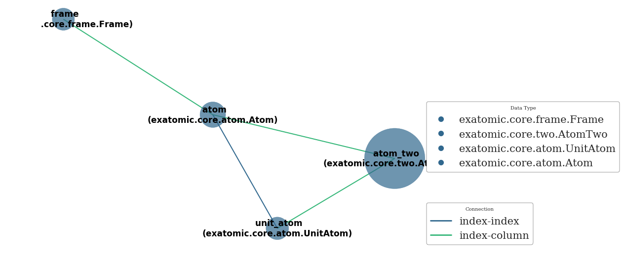
Since atom_two scales quadractically its size is large compared to the other datatables
The unit_atom table is needed for computing periodic two-body data

[20]:

uni.atom_two.dtypes

[20]:

atom0         category
atom1         category
dr             float64
projection       int64
bond              bool
dtype: object

Of course we can also visualize the animation of the trajectory!

[21]:

exatomic.UniverseWidget(uni)

[ ]:

[ ]:

[ ]:

[ ]:

[ ]: